DIII-D Time-Dependent Simulation — FUSE Summer School

This tutorial walks through a complete time-dependent workflow in FUSE for a real DIII-D discharge (shot 200000). Starting from experimental data, we run three complementary cases:

1. Replay: follow the experimental kinetic profiles to reproduce the shot and validate FUSE against the measurements.
2. Simulation: let the physics models predict the profiles (dynamic pedestal + flux-matched transport).
3. Modified simulation: a *"what if?" example with extra electron-cyclotron heating (ECH).

All three share the same configured starting point (:replay_init), so their differences isolate the effect of the modeling choices and the added heating.

What you'll learn

• Fetch experimental data for a DIII-D shot into ini / act
• Initialize dd and checkpoint progress with @checkin / @checkout
• Detect the L–H transition and extract pedestal parameters from experiment
• Run a time-dependent simulation with ActorDynamicPlasma in replay and predictive modes
• Apply synthetic diagnostics and animate the plasma evolution
• Explore a counterfactual with extra ECH

Prerequisites

• A working FUSE install — see the installation guide, or use the GA Omega server
• Access to the DIII-D data system — this notebook fetches shot 200000. If you don't have data access you can still read along: the outputs on this page are pre-rendered.

Companion page: DIII-D Time-Dependent workflows.

1. Load FUSE

We load FUSE together with Plots for figures and Interact for interactive widgets.

The first using FUSE triggers Julia's just-in-time compilation, so it takes a while, while every subsequent call is fast.

# Import needed packages
using Plots;
using FUSE
using Interact
FUSE.ProgressMeter.ijulia_behavior(:clear);

<div style="padding: 1em; background-color: #f8d6da; border: 1px solid #f5c6cb; font-weight: bold;"> <p>The WebIO Jupyter extension was not detected. See the <a href="https://juliagizmos.github.io/WebIO.jl/latest/providers/ijulia/" target="_blank"> WebIO Jupyter integration documentation </a> for more information. </div>

2. Fetch the experiment

FUSE.case_parameters(:D3D, shot) pulls experimental data for a DIII-D shot from the MDS+ data system and returns the 0D initialization parameters (ini) and the actor controls (act). Here we use shot 200000.

We @checkin the result under the tag :fetch, so we can restore this exact starting point later without re-fetching.

use_local_cache=true reuses a previously cached fetch instead of hitting the server — handy when re-running the notebook.

# setup ini, act from MDS+ data
shot = 200000; @time ini, act = FUSE.case_parameters(:D3D, shot; use_local_cache=true)

# save ini, act in case we want to view later
@checkin :fetch ini act;

[ Info: Connecting to mcclenaghanj@somega.gat.com
[ Info: Remote D3D data fetching for shot 200000
[ Info: Path on mcclenaghanj@somega.gat.com: /cscratch/mcclenaghanj/d3d_data/200000
[ Info: Path on Localhost: /var/folders/xw/fh54dglx5h3_mxz2y46jqv9h0000gq/T/mcclenaghanj_D3D_200000
[ Info: Loading files: D3D_machine.json ; D3D_200000_5000167971831672853.h5 ; nbi_ods_200000.h5
actors: FitProfiles
[ Info: Thomson subsystems scaled to match interferometer measurements: TS_core=1.047, TS_tangential=0.958


 74.703604 seconds (371.96 M allocations: 22.948 GiB, 3.58% gc time, 19 lock conflicts, 231.39% compilation time: <1% of which was recompilation)

3. Initialize the data structure

FUSE.init!(dd, ini, act) populates a fresh dd from the experimental data in ini: equilibrium, kinetic profiles, sources, and the actuator pulse schedules. This is our plausible starting state — not yet a self-consistent physics solution.

We checkpoint it as :init so every case below can start from the same point.

# Initialize dd
@checkout :fetch ini act
dd = IMAS.dd()
@time FUSE.init!(dd, ini, act);

# Checkin dd in case we want it for later
@checkin :init dd act;

actors: CXbuild
actors: Sources
actors:  SimpleEC
actors:  SimpleNB
actors:  NeutralFueling


 58.298854 seconds (384.08 M allocations: 25.002 GiB, 3.87% gc time, 90.50% compilation time: <1% of which was recompilation)

4. Analyze the L–H transition

Before evolving the plasma we characterize the pedestal dynamics from the experiment. FUSE.LH_analysis detects the L→H (and H→L) transition times and extracts the quantities the pedestal model needs:

• tau_n, tau_t — density and temperature pedestal build-up timescales
• W_ped_to_core_fraction — how the pedestal stored energy relates to the core
• mode_transitions — the times of confinement-mode changes

With do_plot=true, the detected transitions are overlaid on the experimental traces.

@checkout :init dd act;
experiment_LH = FUSE.LH_analysis(dd; do_plot=true);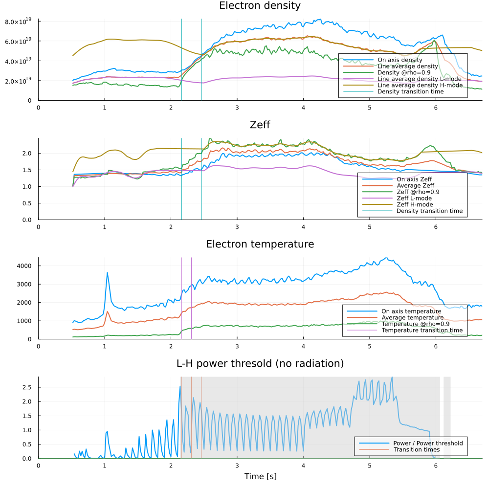

5. Replay: reproduce the shot

In replay mode we follow the experiment: the transport and pedestal actors are set to :replay, so FUSE uses the measured kinetic profiles as boundary conditions while still evolving the current and equilibrium self-consistently. This reproduces the discharge and lets us validate FUSE against the measurements.

Configuration highlights:

• Time stepping — δt = 0.2 s from t = 1.8 s to the end of the equilibrium time base.
• What evolves — current, equilibrium, transport, sources, pedestal, and sawteeth.
• Transport & pedestal — :replay (match experimental values); density and Zeff from experiment.
• Equilibrium — ActorEquilibrium → :FRESCO on a 129×129 grid, constrained by the magnetic diagnostics.

We checkpoint the configured starting state as :replay_init — the shared baseline that the predictive and modified cases below both branch from — then run ActorDynamicPlasma, apply the synthetic diagnostics (ActorMagnetics, ActorInterferometer), and checkpoint the result as :replay.

⏱️ This is one of the expensive cells — it runs a full time-dependent simulation.

# Start from our init dd
@checkout :init dd act;

# setup time
δt = 0.2
dd.global_time = 1.8#ini.time.simulation_start # start_time should be early in the shot, otherwise ohmic current will be wrong
final_time = ini.general.dd.equilibrium.time[end]
act.ActorDynamicPlasma.Nt = Int(ceil((final_time - dd.global_time) / δt))
act.ActorDynamicPlasma.Δt = final_time - dd.global_time

# choose what to evolve
act.ActorDynamicPlasma.evolve_current = true
act.ActorDynamicPlasma.evolve_equilibrium = true
act.ActorDynamicPlasma.evolve_transport = true
act.ActorDynamicPlasma.evolve_sources = true
act.ActorDynamicPlasma.evolve_pf_active = false
act.ActorDynamicPlasma.evolve_pedestal = true
act.ActorDynamicPlasma.evolve_sawteeth = true

# density and Zeff from experiment
act.ActorPedestal.density_ratio_L_over_H = 1.0
act.ActorPedestal.zeff_ratio_L_over_H = 1.0

act.ActorPedestal.mode_transitions = experiment_LH.mode_transitions

# equilibrium model setting
act.ActorEquilibrium.model = :FRESCO 
act.ActorFRESCO.nR = act.ActorFRESCO.nZ = 129

# Particle fueling source rate
act.ActorNeutralFueling.τp_over_τe = 0.5

act.ActorPedestal.rotation_model = :replay # we don't have a good model for the rotation boundary condition

act.ActorSawteethSource.flat_factor = 1.0
act.ActorSawteethSource.period = 0.25 # turn off if no qmin<1 for 250 ms

# Set pedestal and transport to replay to match experimental values
act.ActorCoreTransport.model = :replay
act.ActorPedestal.model = :replay
act.ActorPFactive.boundary_weight = 1.0
act.ActorPFactive.magnetic_probe_weight = 1.0
act.ActorPFactive.flux_loop_weight = 1.0
act.ActorPFactive.strike_points_weight = 0.0
act.ActorPFactive.x_points_weight = 1.0


@checkin :replay_init dd act;

# run time-dependent simulation
@time actor = FUSE.ActorDynamicPlasma(dd, act; verbose=true);
# synthetic diagnostics
FUSE.ActorMagnetics(dd, act)
FUSE.ActorInterferometer(dd, act)
@checkin :replay dd act;

Progress: 100%|███████████████████████████| Time: 0:00:45 ( 0.17  s/it)
       start time: 1.8
         end time: 6.699999809265137
             time: 6.699999809265137
            stage: PFactive (2/2)
          Ip [MA]: 1.180137619570065
        Ti0 [keV]: 1.178052310398543
        Te0 [keV]: 1.7932763995578052
   ne0 [10²⁰ m⁻³]: 0.24647891062974975
        max(zeff): 1.5543193173501326
      ω0 [krad/s]: 21.585265207737137


 55.691934 seconds (167.32 M allocations: 12.802 GiB, 1.64% gc time, 49.14% compilation time: <1% of which was recompilation)


actors: Magnetics
actors: Interferometer

6. Animate the replay

We build an animation of the plasma overview as a GIF. plot_plasma_overview packs the equilibrium, profiles, and heating into a single multi-panel figure. (On this page the animation is shown as a single representative frame.)

# Time basis to step through (one frame per core_profiles time slice).
times = dd.core_profiles.time
@info "Animating $(length(times)) frames" t_start=first(times) t_end=last(times)

fps = 10
anim = @animate for time0 in times
    FUSE.plot_plasma_overview(dd, Float64(time0); aggregate_hcd=true)
end

outfile = joinpath( "./plasma_overview.gif")
g = gif(anim, outfile; fps)

┌ Info: Animating 82 frames
│   t_start = 0.5199999809265137
└   t_end = 6.699999809265137
[ Info: Saved animation to /Users/mcclenaghan/Dropbox/programming/jupyter_notebooks/plasma_overview.gif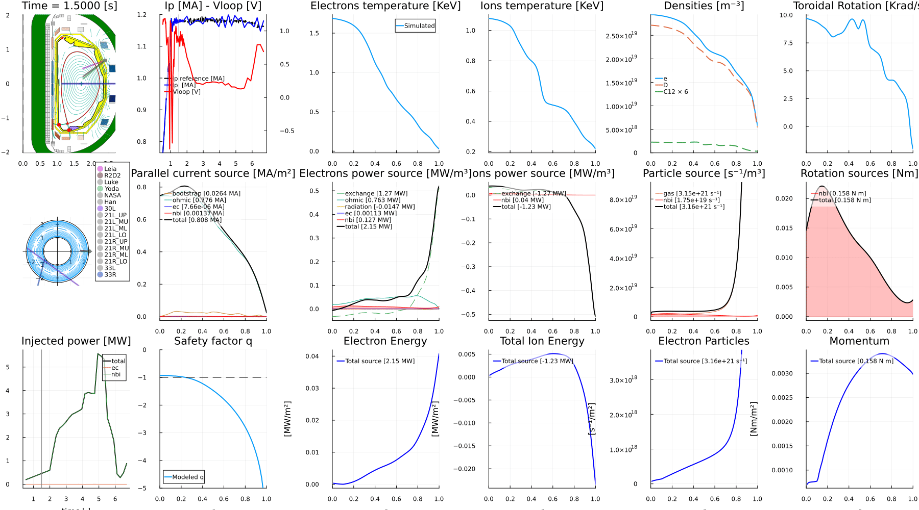

7. Predictive simulation

Now we let FUSE predict the profiles instead of replaying them. Starting again from :replay_init, we switch:

• Pedestal → :dynamic, seeded with the L–H timescales (tau_n, tau_t, W_ped_to_core_fraction) from step 4.
• Core transport → :FluxMatcher, flux-matching Tₑ, Tᵢ, densities, and rotation with ActorTGLF as a :TGLFNN neural-net surrogate.

Running ActorDynamicPlasma now advances the plasma using these predictive models, so the result is a genuine forward prediction rather than a replay of the measured profiles.

@checkout :replay_init dd act;


# Set pedestal model
act.ActorPedestal.model = :dynamic
act.ActorPedestal.tau_n = experiment_LH.tau_n # particle confinement time for LH dynamics
act.ActorPedestal.tau_t = experiment_LH.tau_t # particle confinement time for LH dynamics
act.ActorWPED.ped_to_core_fraction = experiment_LH.W_ped_to_core_fraction
act.ActorEPED.ped_factor = 0.8 # Average pedestal height relative to EPED
act.ActorPedestal.T_ratio_pedestal = 1.0 # Ti/Te in the pedestal

# Set core_transport
act.ActorCoreTransport.model = :FluxMatcher
act.ActorFluxMatcher.evolve_plasma_sources = true 
act.ActorFluxMatcher.algorithm = :simple_dfsane
act.ActorFluxMatcher.max_iterations = -300 # negative to avoid print of warnings
act.ActorFluxMatcher.evolve_pedestal = false
act.ActorFluxMatcher.evolve_Te = :flux_match
act.ActorFluxMatcher.evolve_Ti = :flux_match
act.ActorFluxMatcher.evolve_densities = :flux_match
act.ActorFluxMatcher.evolve_rotation = :flux_match
act.ActorFluxMatcher.relax = 1.0

act.ActorTGLF.tglfnn_model = "sat0quench_em_d3d+mastu_azf+1"
act.ActorTGLF.model = :TGLFNN

@time actor = FUSE.ActorDynamicPlasma(dd, act; verbose=true);
# synthetic diagnostics
FUSE.ActorMagnetics(dd, act)
FUSE.ActorInterferometer(dd, act)

@checkin :predict dd act;

Progress: 100%|███████████████████████████| Time: 0:01:08 ( 0.25  s/it)
       start time: 1.8
         end time: 6.699999809265137
             time: 6.699999809265137
            stage: PFactive (2/2)
          Ip [MA]: 1.169753418712516
        Ti0 [keV]: 2.8721388943358592
        Te0 [keV]: 3.374922254240665
   ne0 [10²⁰ m⁻³]: 0.2725052083379953
        max(zeff): 1.394295077798294
      ω0 [krad/s]: 37.00975617192601


 70.360404 seconds (193.58 M allocations: 18.972 GiB, 2.08% gc time, 57.57% compilation time: <1% of which was recompilation)


actors: Magnetics
actors: Interferometer





ActorInterferometer(dd, par)

8. Modified simulation with extra ECH

Finally, a "what if?". Starting once more from :replay_init, we modify the EC launcher pulse schedule: re-aim all five gyrotrons (via convert_DIII_D_to_IMAS_launch_angles, which maps DIII-D AZIANG/POLANG conventions to IMAS steering angles) and add 0.5 MW per beam after t = 2 s. Rerunning ActorDynamicPlasma shows how the extra electron-cyclotron heating changes the plasma.

# Rerun simulation again with extra EC

@checkout :replay_init dd act;

function convert_DIII_D_to_IMAS_launch_angles(AZIANG, POLANG)
    phi_tor = deg2rad(AZIANG - 180.0)
    theta_pol = deg2rad(POLANG - 90.0)

    steering_angle_tor = -asin(cos(theta_pol) * sin(phi_tor))
    steering_angle_pol = atan(tan(theta_pol), cos(phi_tor))

    return steering_angle_tor, steering_angle_pol
end

for i in 1:5
    # Change launch angles if desired.
    alpha,beta = convert_DIII_D_to_IMAS_launch_angles(200.0, 120.)
    dd.ec_launchers.beam[i].steering_angle_pol[:] .= beta
    dd.ec_launchers.beam[i].steering_angle_tor[:] .= alpha
    
    # Change heating to 0.5 MW per gyrotron and to turn on at 2s
    time = dd.pulse_schedule.ec.time
    dd.pulse_schedule.ec.beam[i].power_launched.reference[time.<2.0] .= 0.0
    dd.pulse_schedule.ec.beam[i].power_launched.reference[time.>2.0] .= 0.5e6
end


# choose what to evolve
act.ActorDynamicPlasma.evolve_current = true
act.ActorDynamicPlasma.evolve_equilibrium = true
act.ActorDynamicPlasma.evolve_transport = true
act.ActorDynamicPlasma.evolve_sources = true
act.ActorDynamicPlasma.evolve_pf_active = false
act.ActorDynamicPlasma.evolve_pedestal = true
act.ActorDynamicPlasma.evolve_sawteeth = true


# run time-dependent simulation
@time actor = FUSE.ActorDynamicPlasma(dd, act; verbose=true);
# synthetic diagnostics
FUSE.ActorMagnetics(dd, act)
FUSE.ActorInterferometer(dd, act)

@checkin :predict_modify dd act;

Progress: 100%|███████████████████████████| Time: 0:00:33 ( 0.12  s/it)
       start time: 1.8
         end time: 6.699999809265137
             time: 6.699999809265137
            stage: PFactive (2/2)
          Ip [MA]: 1.179880257191097
        Ti0 [keV]: 1.178052310398543
        Te0 [keV]: 1.7932763995578052
   ne0 [10²⁰ m⁻³]: 0.24647891062974975
        max(zeff): 1.5543193173501326
      ω0 [krad/s]: 21.585265207737137


 35.631565 seconds (43.09 M allocations: 6.755 GiB, 2.14% gc time)


actors: Magnetics
actors: Interferometer





ActorInterferometer(dd, par)

9. Compare

We plot the plasma overview at t = 2.5 s, including the rotation profile. Compare it against the replay animation from step 6 to see the effect of the extra heating.

FUSE.plot_plasma_overview(dd, 2.5;aggregate_hcd=true, rotation_quantity=:sonic)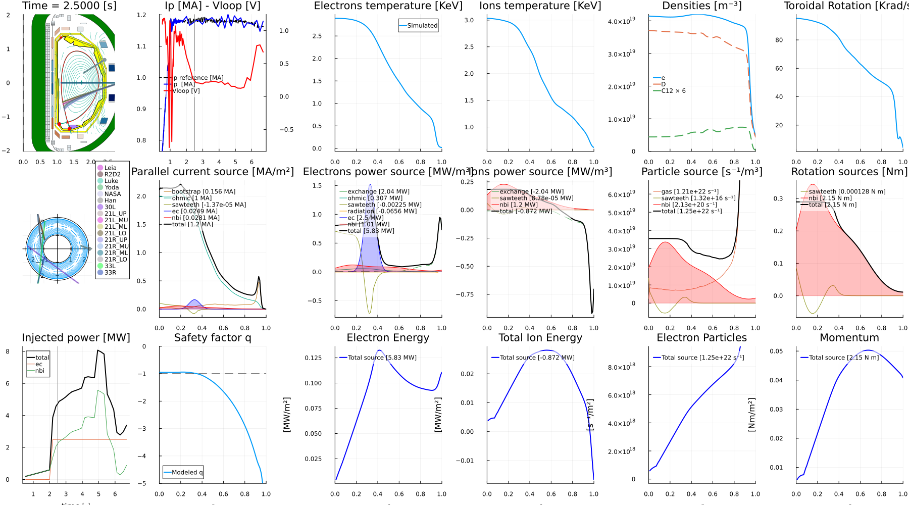

Next steps

• Swap the shot number to run your own DIII-D discharge
• Compare the replay, predictive, and modified runs using the @checkout checkpoints (:replay, :replay_init)
• Explore the individual physics/engineering models in the Actors documentation
• Learn the core data structures (ini, act, dd) in the introductory tutorial

Acknowledgements

Work supported by US DOE under DE-FC02-04ER54698.